A convenient way to provide such a spectral transformation is to note that
Thus
A moments reflection will reveal the advantage of such a spectral transformation.
Eigenvalues that are near will be transformed to
eigenvalues that are at the extremes and typically
well separated from the rest of the transformed spectrum. The corresponding eigenvectors
remain unchanged. Perhaps more important is the fact that eigenvalues far from the
shift are mapped into a tight cluster in the interior of the transformed spectrum.
We illustrate this by showing the transformed spectrum of the matrix ![]() from
Figure 4.8 with a shift (here ).
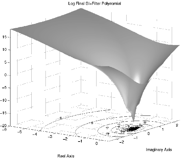
Again, we show the total filter polynomial that was constructed during an IRA iteration
on the transformed matrix . Here we compute the six eigenvalues of largest magnitude. These will transform back to eigenvalues of
from
Figure 4.8 with a shift (here ).
Again, we show the total filter polynomial that was constructed during an IRA iteration
on the transformed matrix . Here we compute the six eigenvalues of largest magnitude. These will transform back to eigenvalues of ![]() nearest to
through the formula .
The surface shown in Figure 4.9 is again but
plotted over a region containing the spectrum of .
Here, is the
product of all of the filter polynomials constructed during the course
of the iteration. Since the extrem eigenvalues are well separated the
iteration converges much faster and degree of is only 45 in this case.
Here, the ``+" signs are the
eigenvalues of in the complex plane and the contours are the level curves
of . The circled plus signs are the converged eigenvalues.
The figure illustrates how much easier it is to isolate desired eigenvalues after a spectral
transformation.
nearest to
through the formula .
The surface shown in Figure 4.9 is again but
plotted over a region containing the spectrum of .
Here, is the
product of all of the filter polynomials constructed during the course
of the iteration. Since the extrem eigenvalues are well separated the
iteration converges much faster and degree of is only 45 in this case.
Here, the ``+" signs are the
eigenvalues of in the complex plane and the contours are the level curves
of . The circled plus signs are the converged eigenvalues.
The figure illustrates how much easier it is to isolate desired eigenvalues after a spectral
transformation.
If ![]() is symmetric then one can maintain symmetry in the Arnoldi/Lanczos
process by taking the inner product to be
is symmetric then one can maintain symmetry in the Arnoldi/Lanczos
process by taking the inner product to be
If ![]() is singular
then the operator has a non-trivial null space and the bilinear
function is a semi-inner product and
is a semi-norm. Since is assumed to be
nonsingular,
Vectors in are generalized eigenvectors corresponding to infinite eigenvalues.
Typically, one is only interested in the finite eigenvalues
of () and these will correspond to the non-zero eigenvalues of S.
The invariant subspace corresponding to these non-zero eigenvalues
is easily corrupted by components of vectors from during the Arnoldi process. However, using the M-Arnoldi process
with some refinements can provide a solution.
is singular
then the operator has a non-trivial null space and the bilinear
function is a semi-inner product and
is a semi-norm. Since is assumed to be
nonsingular,
Vectors in are generalized eigenvectors corresponding to infinite eigenvalues.
Typically, one is only interested in the finite eigenvalues
of () and these will correspond to the non-zero eigenvalues of S.
The invariant subspace corresponding to these non-zero eigenvalues
is easily corrupted by components of vectors from during the Arnoldi process. However, using the M-Arnoldi process
with some refinements can provide a solution.
In order to better understand the situation, it is convenient to
note that since ![]() is positive semi-definite, there is an orthogonal
matrix such that
is positive semi-definite, there is an orthogonal
matrix such that